
A straight line is often the first forecast we try. Plot monthly output, fit a trend through the observations, and extend it six months. The result is easy to explain. It can also be confidently wrong.
Forecasting asks a specific question: given what we know today, what range of outcomes should we expect at a future date? That differs from a target (what we want) and a plan (what we will do). A production target of 100,000 tonnes next month is not a forecast merely because it appears in a budget. If recent throughput, planned maintenance and ore characteristics imply 88,000–96,000 tonnes, the gap calls for a decision, not a more optimistic trend line.
Start with the decision
Before choosing a model, specify four things:
- What quantity? Daily plant throughput, weekly work orders, hourly power demand or monthly sales?
- How far ahead? Tomorrow’s shift roster may need a one-day forecast; procurement may need three months.
- When is the forecast made? A forecast issued Friday cannot use the actual rainfall or breakdowns recorded next Tuesday.
- What does an error cost? Underestimating spare-parts demand may stop production; overestimating it may tie up cash.
The same dataset may need different forecasts for different decisions. Forecasting total tonnes for a monthly executive report is different from forecasting hourly feed to schedule a plant.
Why linear regression is a useful starting point
Suppose weekly output over 20 weeks rises gradually. A regression of output on week number fits a line:
Forecast output = starting level + weekly change × future week.
It provides a clear baseline. If the process truly has a stable linear trend and no meaningful recurring pattern, that may be enough. But the line treats each week as part of one continuing slope. It does not automatically know that Sundays differ from weekdays, that a shutdown is scheduled, or that a step change occurred after a new crusher came online. Extending a recent improvement indefinitely can produce physically impossible output.
The next step is to identify which repeatable information the line misses and test whether adding it improves forecasts.
Three practical examples beyond the line
1. Demand repeats by day and season
Imagine electricity demand for an industrial site: weekdays are busy, weekends are quiet, and hot afternoons increase cooling load. A line through the hourly observations will miss much of this structure.
Start with a seasonal naïve forecast: predict next Monday at 2 pm using a comparable Monday at 2 pm. Then compare a model that accounts for time of day, day of week and expected temperature. If tomorrow’s temperature forecast is uncertain, show how that uncertainty affects the demand forecast.
The key is to compare methods against a simple seasonal baseline. A sophisticated model that cannot beat “same time last week” has not earned its complexity.
2. A shutdown creates a break in the series
Suppose monthly plant output has risen for a year, but a ten-day shutdown is already scheduled next month. Extrapolating the historical slope ignores information available when the forecast is issued.
Forecast operating days and expected output per operating day, then combine them. If there are 20 planned operating days and a plausible 4,200–4,600 tonnes per day, the operating-range calculation is 84,000–92,000 tonnes before allowing for startup losses and unplanned downtime. Those numbers are illustrative.
A time-series model can describe normal behaviour; a known shutdown needs an explicit adjustment or predictor. Document the assumption so the forecast can be revised if the schedule changes.
3. Conditions change after equipment is replaced
A pump’s weekly vibration readings might hover near 4 mm/s, then settle near 2 mm/s after bearing replacement. A regression fitted across both periods can imply a steady downward trend, although the process may simply have moved to a new level.
For forecasting, mark the intervention date. Check whether the post-repair readings form a stable new regime and whether there are enough observations to estimate it. For fault detection, the task is different: forecast normal readings under current conditions and investigate meaningful departures. Do not treat the old high readings as evidence that vibration must keep declining.
Worked example: forecasting next week’s output
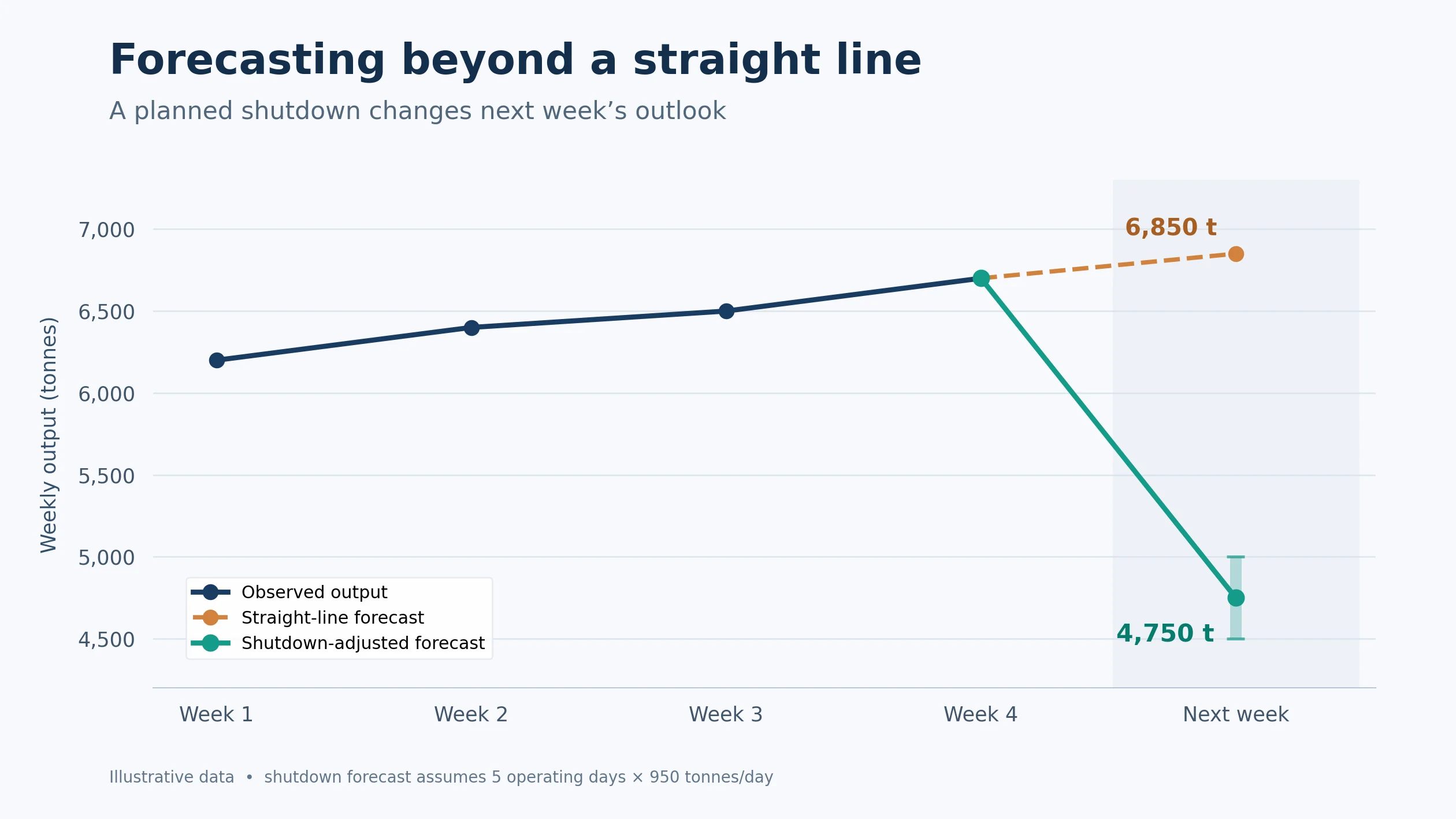
A plant produced 6,200, 6,400, 6,500 and 6,700 tonnes over the last four weeks. A straight-line trend suggests roughly 6,850 tonnes next week. That looks reasonable until the maintenance schedule shows the plant will run for only five of its usual seven days.
Suppose recent production on operating days averaged 950 tonnes. A schedule-aware starting forecast is 5 days × 950 tonnes = 4,750 tonnes. If operating-day output has recently ranged from 900 to 1,000 tonnes, that gives an illustrative 4,500–5,000-tonne operating range. This range is a scenario calculation, not a statistically calibrated prediction interval; unplanned downtime could lower the result further.
Now compare both approaches with earlier weeks that had planned stoppages. At each earlier forecast date, use the maintenance schedule as it stood then. If the schedule-aware method consistently has smaller errors, use it. If it fails when restarts are slow, add a startup allowance and test again. The value comes from matching the forecast to what the business knew at the time, not simply fitting a more elaborate curve.
Which methods should you try?
| Pattern or constraint | Useful first candidates | What to check |
|---|---|---|
| Little visible structure | Latest value or historical average | Does the simple forecast hold up out of sample? |
| Repeating weekly or annual cycle | Seasonal naïve, seasonal exponential smoothing | Is the cycle stable and represented in the history? |
| Changing level or trend | Exponential smoothing, ARIMA | Are changes persistent, and do forecasts remain plausible? |
| Known future drivers | Regression with calendar, weather or planned events; dynamic regression | Were those future inputs actually available when the forecast was made? |
| Many related products or sites | Separate forecasts with consistent totals | Do item forecasts reconcile with the aggregate needed for decisions? |
These are candidates, not a ranking. The best method depends on the series, forecast horizon and decision. Even a well fitted explanatory regression needs future values of its predictors; if those are unknown, they must be forecast too or expressed as scenarios.
Test the forecast as it would be used
A random train/test split mixes past and future and can make a forecasting model look better than it is. Instead, choose historical forecast origins. At each origin, train using only information available then, forecast the required horizon, and compare with the later actuals. Repeat across several origins.
For example, if the business needs four-week-ahead forecasts each Friday, simulate that exact process across earlier Fridays. Compare the straight line, seasonal naïve method and one or two relevant alternatives on the same dates and horizons. Report errors in units the user understands, such as tonnes, megawatt-hours or dollars. Inspect whether errors are consistently high during shutdowns or low after a process change.
A forecast should also communicate uncertainty. “90,000 tonnes” suggests precision that may not exist. “Around 90,000 tonnes, with an estimated 80% prediction interval of 83,000–97,000 under the stated operating assumptions” makes the decision risk visible. That interval is an illustration, not a calculated result. A real interval needs to be estimated and checked against historical forecast errors; exceptional events may still fall outside it.
A practical first workflow
- Write down the decision, target variable, horizon and exact forecast issue time.
- Plot the time series. Look for gaps, outliers, cycles, step changes and impossible values; ask operators what changed.
- Establish a naïve or seasonal naïve baseline.
- Add one method suited to the observed pattern, and known future events where justified.
- Run historical forecasts using only information that existed at each issue time.
- Compare errors, review failures and choose the simplest method that meets the decision’s needs.
- Publish the forecast with its assumptions and uncertainty; refresh it as new data arrive.
The lesson beyond simple linear regression is straightforward: time has structure, operations change, and the future is uncertain. Forecasting becomes useful when the model reflects those facts, survives a realistic historical test and helps someone make a better decision.
James is a data and analytics leader with experience across mining, property technology and financial services. He specialises in turning complex operational data into clear insights, better decisions and measurable business value.
He currently leads the delivery of operational performance data products at BHP. His technical skills include Python, SQL, Power BI, Snowflake and AWS, alongside data engineering, automation and cloud application development. James combines hands-on technical work with stakeholder engagement and team leadership, with a growing focus on operational time series analysis, AI and asset intelligence.